Recent Posts

Blog Post 5: Design Reflections of Whispering Woods

I collected my initial data on September 23, 2019; most of the collecting went smoothly and as planned, but during the collection and upon reflection some of it requires modification.

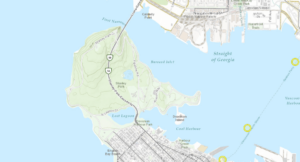
One of these difficulties was my sampling strategy. I had planned on using a systematic sampling strategy (explained in my Small Assignment 1) where I would use a random number generator to indicate which initial tree I would sample (at the very top and bottom row of trees on the hill). From there, I would count 9 trees, and 18 trees to the left and right of the initial sample to collect a total of 5 replicates. I realized while I was there; however, that if the randomly generated number was very small or very large, there may not be enough trees on one side of that tree to collect the second and third sample. I decided I would instead count another 9 (or 18, if necessary) trees after the 18th tree on the other side, to make up for this. I am having difficulties determining if this modified method of systematic sampling is “random” enough, yet I can’t think of an alternative.

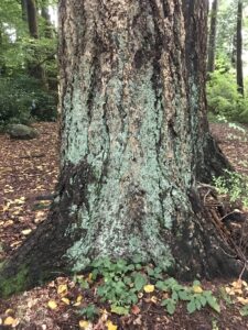
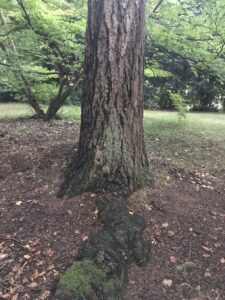
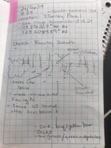
With regards to the actual data I collected, the mean soil moisture levels at the bottom and top of the hill followed my prediction (the bottom of the hill having a higher mean moisture level). My leaf class strategy (class 1 being trees with 0-5% yellow leaves, class 6 being trees with 95-100% yellow leaves) will likely become more useful as the Fall progresses, as the vast majority of trees at the top and bottom of the hill all fell under the class 1 category. As well, the soil pH readings were very similar at both locations along the elevation gradient, not providing any useful measurements at the moment.

None of this is surprising, as the data I am collecting is likely to change drastically as the Fall progresses. For instance, we are now in our second day of snowfall in Calgary, Alberta, so it should be interesting to study the differences in soil moisture, pH, and leaf colour later this week after a few days of melting. For this reason, I plan to continue the same measurements as in my initial collection to allow for potential changes in pH, soil moisture, and leaf colour to be captured.

However, there are a few modifications to my data collection I would like to make. Firstly, I would like to adapt my data collection to the seasonal progression changes. For instance, as the Fall progresses I will likely add in a leaf loss measurement similar to my leaf class strategy. This way, I can measure the rate of leaf loss on top and bottom hill trees, which will be more applicable than leaf colour at that point. I may add other measurements as well (such as snow depth, to measure water infiltration rate). I also do not want to stick to a specific schedule as to when I collect data. Of course, data collection must be frequent enough to be able to capture changes in the health parameters I’ve mentioned, but I would also like to respond to weather changes. For instance, I will not be collecting data while the location is buried in 1ft of snow, as my pH and moisture meter do not have the capabilities to function in such drastic conditions. Instead I will collect data soon after the snow has melted, to study initial differences among the elevation gradient. Ideally, I would like to collect data no more frequently than every 5 days, but no less frequently than every 10 days (if weather permits).

I believe these modifications will improve my research because they will account for the natural and uncontrollable fluctuations in weather. Modifying the data I will be collecting will allow for my data to stay relevant as the Fall season progresses. Modifying the frequency of data collection will achieve the exact same thing. I hope, through these modifications across time, that I will more holistically be able to capture any differences in tree health among trees located at the bottom and top of Whispering Woods hill.

That’s all for now!

Madeleine Browne

Academic Peer-Reviewed Research Article Example

a.) The ecological information source I selected for this exercise is the following journal article:

Hamann, A. & Wang, T. (2006). Potential effect of climate change on ecosystem and tree species distribution in British Columbia. Ecology 87(11), pp. 2773-2786. Retrieved from http://www.jstor.org.ezproxy.tru.ca/stable/20069297

b.) This article is classified as academic peer-reviewed research

c.) It was written by experts in the field, employed by the University of British Columbia, at the Centre for Forest Gene Conservation within the Department of Forest Sciences. It has in text citations (ie. p. 2773) and contains a bibliography (p. 2784). It has been peer-reviewed by at least one referee based on the description in the acknowledgements (p. 2784) and the description of manuscript revisions and acceptance (p. 2773). It reports laboratory results, and contains a methods and results section indicating it is research based. Additionally, the methods and results report their own data collection, processing, and findings, affirming the article is research-based. For these reasons, this article would be considered an academic peer-reviewed research article.


Preliminary Observations and Interests in Stanley Park

The location I have chosen to study is Stanley Park, in Vancouver. Stanley Park is an urban public park that covers 404.9 hectares, located in the lower mainland region of British Columbia. The park is situated between downtown Vancouver (south), and the ocean water of Burrard Inlet and English Bay (north, east, and west; Photo 1).

Photo 1. Aerial image of Stanley Park (Image retrieved from Google Earth Pro)

The elevation ranges from sea level to 76 m throughout the park (Photo 2). Prospect point located in the northern part of the park, is the topographic peak of the park. The vegetation within Stanley Park consists primarily of forest (conifers and deciduous). The Vancouver city park is located on Federal land that is leased  to the City of Vancouver, and was established in 1888 by Lord Stanley.

Photo 2. Topographical base mapping of Stanley Park (Image retrieved from from iMap BC).

On 24 September 2019 I observed a small area of the forest (100m line of trees North to South; Photo 3 – 5) in the southeastern corner of the Park (Photo 6). I visited from 18:23 to 19:00, before sunset (19:05). The weather and general site conditions consisted of low light, light wind, and 14°C.

Photo 3. Base of Douglas fir (Pseudotsuga menziesii) with visible dust lichen (Lepraria species) and moss (unidentified)
Photo 4. Base of Douglas fir (Pseudotsuga menziesii) showing multiple types of unidentified moss and lichen on exposed root bark.
Photo 5. Field notes 24 September 2019 describing general forest observations


Photo 6. Approximate location of observation for Module 1 Observations (Image retrieved from Google Maps)


Potential subjects of study:

  • Trees (ie. coniferous and/or deciduous)
  • Mosses
  • Lichens

Potential research questions:

  1. What physical conditions in Stanley Park favour the growth of lichen and/or moss on trees?
  2. Is there a pattern of distribution of lichen and/or moss species across Stanley Park?
  3. Does lichen and/or moss grow on all tree species in the Stanley Park?

Sources:

B.C. Conservation Data Centre: CDC iMap [web application]. 2019. Victoria, British Columbia, Canada. Available: http://maps.gov.bc.ca/ess/sv/cdc/ (24 September 2019).

Google. (n.d.). Stanley Park. Retrieved from: https://www.google.com/maps/place/Stanley+Park/@49.3064903,-123.1521274,14.38z/data=!4m5!3m4!1s0x5486718cad26e4a3:0x364a639db409e216!8m2!3d49.3042584!4d-123.1442522

Blog Post 9: Field Research Reflections

I didn’t have too much trouble implementing my design, however it was maybe too simple. The data ended up being quite difficult to analyse and if I had larger sample sizes, there may have been a more apparent trend. This is the first research project I’ve carried out on my own, so that was much harder than I expected since I had no one to bounce ideas off of as I saw how things played out. The more I learn, the more complicated ecological theory becomes. I am eager to keep working in this field and to continue learning how to design effective and efficient experiments.

Post 4: Sampling Strategies

In the online sampling simulation, I chose to sample the Mohn Mill site using distance sampling. I found that systematic distance sampling had the fastest estimated sampling time with 4 hours and 7 minutes.

The percent error for species density of the two most common and two rarest species at the Mohn Mill site using distance systematic sampling is as follows:

red maple = |(392.4-403.7)/403.7|x100 = 2.799%

white oak = |(49.9-74.5)/74.5|x100 = 33.0%

yellow birch = |(0.0-0.8)/0.8|x100 = 100%

white ash = |(0.0-0.8)/0.8|x100 = 100%

The percent error for species density for the same species as above using distance random sampling is as follows:

red maple = |(380.8-403.7)/403.7|x100 = 5.673%

white oak = |(53.3-74.5)/74.5|x100 = 28.5%

yellow birch = |(7.6-0.8)/0.8|x100 = 850%

white ash = |(0.0-0.8)/0.8|x100 = 100%

The percent error for species density for the same species as above using distance haphazard sampling is as follows:

red maple = |(735.5-403.7)/403.7|x100 = 82.19%

white oak = |(157.6-74.5)/74.5|x100 = 112%

yellow birch = |(0.0-0.8)/0.8|x100 = 100%

white ash = |(0.0-0.8)/0.8|x100 = 100%

The more abundant the species, the more accurate the sampling. Conversely, the less abundant the species, the less accurate the sampling.

Systematic sampling appears to be the most accurate sampling method, followed by random sampling, and finally haphazard sampling.

BLOG POST 8

So far I have made two graphs:

  1. The correlation between the number of pollinators and the temperature
  2. The relationship between the number of pollinators and the amount of precipitation (mm)

I think both of these graphs are perfect for showing my data that I have collected. I think my data is all normal, obviously it would be better had I recorded data for a longer period of time.


Post 2: Sources of Scientific Information

The article “Himalayan wolf foraging ecology and the importance of wild prey” is from Science Direct, and was published in 2019 by Elsevier B.V. on Global Ecology and Conservation.

The article can be found here:

https://www.sciencedirect.com/science/article/pii/S2351989419301830

This article is academic peer reviewed research material containing in-text citations and a bibliography on the page 12. It is written by eight experts who work in various organizations as stated on the top of the first page. On the home page the Elsevier Journal it states that all articles hosted on Science Direct are peer reviewed (https://www.journals.elsevier.com/global-ecology-and-conservation), and on the first page of the article in the “Article Info” section also states that the article has been revised. This article is a field study and contain a “Methods” and “Results” section on pages 2-4. 

Post 1 – Observations

Blog Post 1 – Observations

The location I have chosen to study is along Coquitlam River Trail on the Port Coquitlam side. It is a large area spanning many kilometres, but I have chosen a plot of about 75m X 75m. Weather was cloudy, 19 degrees with no visible wind. Area was visited on September 7th 2019 at 15:00-16:30. It features a large river, flowing moderately with clear greenish brown water. In the river is a small rock dam, most likely built by humans. In this area there is less water flow and about 15 bugs are present on the waters surface.  Lining the river are large elm trees and shorter plants with large and flat green leaves. These shorter plants host many spiders in their webs. Western sword fern are approximately 4-5 metres from the rivers edge on a higher bank. Pine and maple trees are in the same area, and are more present further back into the forest. Trees with flat branches and soft needles are present as well – possibly hemlock. One log on the rivers edge is covered in Oyster mushrooms, including one large one about 20cm long. No other logs nearby have these mushrooms present. There are a few small paths going into the forest with trampled vegetation, possibly from humans, dogs, bear, coyote or deer. Birds can be heard but not seen.

Questions arising from this observation:

Why are the Oyster mushrooms only on this one log?

Why are most of the Elm trees leaning towards the river?

I noticed that the larger trees are beginning to change colour, but the shorter shrubs and younger elm are not. Is there a reason for this?

The river bed contains sand and large rocks, but nothing in between. Why are there no smaller stones present? And why do only the rocks on shore have moss, not ones that are partially in the river?

Why are there no maple trees near the rivers edge?

Do only certain plants survive near the rivers edge?


BLOG POST 7

My main focus has been if there is a correlation between the number of pollinators and the weather. I have done this at a garden that has plant species that are to attract bees, therefore in theory there should be a fair number of bees in this general area. This can also tie in with the temperature of the day, the humidity, the wind, there are honestly all kinds of other factors that can affect the results. I am taking the temperature of the day and the type of weather into consideration when I am counting the number of pollinators in/ near the garden.

Three keywords for my research could be pollinators, botanical gardens, weather.

Post 3: Ongoing Field Observations

I plan to study the Douglas Fir trees found at the junction of Johnny’s trail and Douglas Fir trail in Canmore, AB.

Notable locations along the environmental gradient of my location include: a flat, open forested area; a more densely forested area on a slope; and a rocky, sparsely vegetated spring run-off gully.

The first location has a variety of shrubbery, clover, and rose bushes; along with randomly dispersed Douglas fir trees in low abundance. The trees appear to grow as individuals. On average, there appears to be more Douglas fir saplings in comparison to older trees. All Douglas fir trees present appear to have branches evenly dispersed around the tree’s radius.

The second location has less of a variety of shrubbery, clover, and rose bushes. There are more densely dispersed Douglas fir trees in great abundance. The trees appear to grow in clumps. There appear to be more older trees than saplings.

The third location has very few plants. There are a few immature Douglas fir trees growing around the edges of the gully, along with a few shrubs. The Douglas fir trees grow alone and are nearly all older trees. The trees are widely dispersed and in low abundance.

My hypothesis I wish to test is as follows: do Douglas fir trees better resist cooling temperatures of changing seasons in groups or as individuals? I predict that the trees will fair better against the temperature change in groups.

A possible responding variable is the abundance, distribution, and size of the Douglas fir trees in each location. This variable is continuous. A possible predictor variable is the ambient air temperature and weather. This variable is also continuous.