Recent Posts

Post 1: Observations

Just north west of Fort St John, BC,  lies Charlie Lake. From the southern tip of this lake runs Fish Creek. Fish creek is a small creek that runs approximately 14 km, flowing first south east and then turning northeast to flow in to the Beatton River. I have chosen to observe a roughly 2.5 km section of the creek about 3/4 of the way along it’s path towards the Beatton River (Google Maps, 2019). The above measurements are very rough estimates.

In the area I have chosen for study, Fish Creek snakes its way through a rather steep gully. I visited the area on 19-11-17 at approximately 1510 until 1630. It was unusually warm for November at 9 degrees Celsius. It was quite windy (I guessed it was 30 km/hr gusting 50 km/hr out of the south west) but sunny. I will try to remember to bring my Kestrel next time to get a more accurate weather reading.

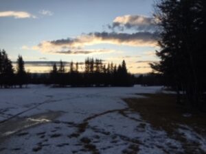
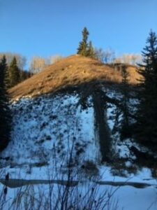
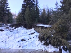
On the south facing bank of the gully itself the flora is predominantly grassy with some smaller shrubs, most likely Prickly Rose (Rosa acicularis). At the top of the slope on that south facing side there stands mostly Trembling Aspen (Populus tremuloides). Behind that lies farmed crop fields (these fields will not be included in my study as they are private land). At the bottom of both sides of the gully, directly adjacent to the creek, there are flat, sort of swampy areas with Prickly Rose and what I am pretty sure is Blue Wildrye (Emlymus glaucus), though it is hard to tell at this time of year, and a “willow” shrub that I do not know the name of, though it has been on my list of plants to learn for a while now. What I do know is that moose love it as a forage. I have observed in many other locations the tops of this shrub neatly snipped off by the big mammals.  The north facing slope is predominantly a stand of mature White Spruce (Picea glauca) with the odd Paper Birch (Betula papyrifera) and Trembling Aspen. The under story is mostly Blue Wildrye and Prickly Rose (making it somewhat unpleasant to walk through). There are pockets of Trembling Aspen stands on mid slope benches. At the top of the north facing slope there is a band of mixed trees, though most are Trembling Aspen. Behind this there lies a golf course. I will be including this grassy course in my study area as I access the Fish Creek gully (which is Crown Land) via the public path through the golf course. I access the lower part of the gully via a pipeline right of way that runs straight down the north facing bank and then up the south facing bank on the far side. The right of way is open grass with some White Spruce regeneration.

Pipeline Right of Way
Golf Course (looking west)


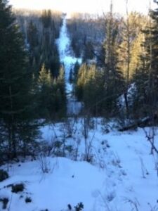
One observation I noted was the difference in apparent slope instability between the north facing and south facing slopes. There is fairly abundant evidence of slides and slope instability on the south facing slope at all levels. On the north facing slope, there is considerably less, though still some evidence down low. Perhaps this has to do with the north facing slope having a gentler pitch and mid level benches? Perhaps the presence of White Spruce provides better stability? Maybe because snow melts faster due to sun exposure on south facing slopes (Williams, 2018) the slope becomes saturated and is more prone to slide? I would be very curious to look in to the relation between the south facing slope and its apparent instability.

South facing slope (instability present)
Northern bank instability along creek

I saw one Common Raven (Corvus corax), but no other live animals. I have seen many Red Squirrels (Tamiasciurus hudsonicus) in the general area and was therefore surprised to not see any on this visit. I find these little squirrels very endearing and will be keeping an eye open down there for them. What do they do in the winter in this area? Do they prefer the White Spruce to the Trembling Aspen? Do they prefer the slopes or the flat lands? I imagine that they go in to hibernation for the winter months, but I do not actually know that for a fact.

In the grass land up top, I observed (and have many times in the past while in the area walking my dogs) heavy traffic by Mule Deer (Odocoileus hemionus), as evidenced by their hoof prints in the snow. I was expecting to follow their trail all the way down the pipeline right of way to the bottom of the gully and then along the creeks edge. They did not appear to go all the way down though, and I am not sure at which point they veered from the right of way. This is a question that I am very interested in researching. What are the winter traffic patterns of Mule Deer in the area? Where do they bed down? Where do they feed? Do they prefer the open south facing slopes to the flat golf course? How does snow pack affect their behavior? I chose my area of study knowing that Mule Deer frequent the area and will likely base my research on their patterns in this area, where man-made field meets forest and gully.

Mule Deer tracks

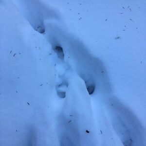
I also noticed several Canine tracks in the snow on the pipeline and down at the bottom of the gully. There were many sets of tracks, traveling along the creek’s edge and crisscrossing it. There appeared to be different size of tracks. Perhaps Red Fox (Vulpes vulpes) or Coyote (Canis latrans)? I am confident they are not some one’s dog as the area in the gully has no paths or human traffic (aside from me) evident. I am interested to understand more about these canine’s travel patterns though the area. It would be interesting to find out if they prefer to run over the frozen creek (when it does freeze), or on the flats beside the creek. Does snow depth or slope have an effect? Does the presence of these canine’s affect the Mule Deer in the area?

I have started these observations at a good time of year as the season is shifting from fall to winter. I will be using this seasonal change to help me focus my study.


Sources:

Google Maps. (2019). Retrieved November 20, 2019, from https://www.google.com/maps/@56.278364,-120.8526553,7633m/data=!3m1!1e3

Williams, D. (2018). Differences Between North- and South-Facing Slopes. Retrieved November 20, 2019 from https://sciencing.com/differences-between-north-southfacing-slopes-8568075.html


Blog Post 7: Theoretical Perspectives

My research project aims to validate a pattern I observed, that Common snowberry (Symphoricarpos albus) distribution is limited to environments with less than 20% slope gradient, or that common snowberry distribution diminishes as slope gradient percentage increases. During my initial field observations, I started noticing that plant species occurred in one environmental gradient, but not in the other. My first observation was that the dominant tree species would differ between environmental gradients. For example, the riparian area was dominated by black cottonwood (Populus trichocarpa), whereas the upland area was dominated by ponderosa pine (Pinus ponderosa). When I started making observations about the shrub and herb layer I noticed similar patterns, where some species were present in one area, but not in the other.

I chose to focus on common snowberry distribution and started asking questions that may explain why common snowberry was present in the riparian area, but not in the upland area. I questioned slope gradient percentage as a potential indicator of water availability, slope aspect as an indicator of sun exposure, soil type, soil moisture and surrounding topography. When I relate this back to ecological processes, I want to focus my research project on abiotic factors and the physical environment including local topography, the hydrological cycle and the energy cycle. In summary, my research aims to explore that the physical environment (topography, slope, aspect etc.) is an indicator of species occurrence and ecological communities.

Three keys words I would associate with my research project include, ecosystem indicators, ecological communities and physical environment.

Post 9: Field Research Reflections

I really struggled with this course overall. I had a difficult time creating a hypothesis. I had a hard time making sure that my hypothesis and study was even tangentially related to ecology as I have absolutely no background in ecology at all. I was challenged to trust my results as I felt that it would take a much longer study period to really and truly make valid conclusions. The main issue that came up with implementing my field study was being available during the same time period every day. There were a few days that were missed due to work schedule changes that had me travelling out of the city or my parents forcing me to attend Thanksgiving dinner. I was lucky in that I was able to recruit an assistant (my husband who is contractually obligated to help me out, as stated in our vows) to attend a few days for me while I was away at a conference for 5 days. Overall, were I to attempt this study again, I would like to set up a remote monitoring system that would allow for 24 hour tracking for a full year to really gather a full sense of the variables that affect the populations of the park. I have so much appreciation for anyone who practices ecology as their knowledge and commitment far exceeds my own.

Post 6: Data Collection

I have been attending Mill Lake Park nearly every day between 17:30-17:45 to gather weather and population data. So far, I have attended 37 days since September 10th having missed 4 days in that period. The main difficulty has been ensuring that I was available during the time period every day. I’ve noticed significant changes in the populations with subjective declines in weather conditions. I predicted that fewer people would visit the park on days of inclement weather, but I had not initially anticipated that those who did visit on the poor weather days would be predominantly accompanying a dog. Upon further reflection, it made sense to me that those who had to walk their dog would be less inclined to remain inside out of obligation to their pet.

Post 5: Design Reflections

My sampling strategy was overall pretty easy to implement. The main difficulty that I ran in to was trying to be at the park every day during the same time period. There were a few days that were missed due to traffic conditions on the drive home when I was transferred to a different location for work. There were also a few days were I was at the World Sleep Symposium where my husband went to the park on my behalf but there were some inconsistencies with his measurements compared to mine that I suspect are user error differences.

One difficulty that I’m foreseeing if I continue to collect data is the upcoming time change as well as sunset rapidly descending upon my collection time. Currently I’m measuring from 17:30-17:45 every day. Sunset is currently at 18:08 and gets a few minutes earlier each day. I anticipate that the darkness will drastically change my collection numbers and I’m unsure if I should continue a 24 hr cycle of measurement after the time change and measure at 16:30-16:45 or if I should stay with the accepted clock time. These may not come up as I anticipate that I will stop collecting data before the time change, as far as it pertains to this report, though I may continue on my own accord out of sheer curiosity.

Post 4: Sampling Strategies

For the virtual sampling exercise, I sampled from the Snyder-Middleswarth Natural Area. I utilized random, systematic, and haphazard sampling strategies. Of these, the systematic was the most time efficient clocking in at 4hrs and 5 minutes, though the haphazard was a close second at 4 hrs 27 minutes compared to the random strategy which took 12 hours and 34 minutes.

There was no method that I found to be particularly accurate in its estimation. I calculated error rates for each tree species rather than just the 2 most common and 2 rarest in an attempt to narrow down the “best” method but was still left with few answers.
My error calculations showed:
Eastern Hemlock (actual density 469.9) – Random – 3.3%; Systematic – 22.2%; Haphazard – 3.6%
Sweet Birch (actual density 117.5) – Random – 31.2%; Systematic – 11.7%; Haphazard – 60.9%
Yellow Birch (actual density 108.9) – Random – 57.9%; Systematic – 55.0%; Haphazard – 9.6%
Chestnut Oak (actual density 87.5) – Random – 52.3%; Systematic – 14.3%; Haphazard – 47.0%
Red Maple (actual density 118.9) – Random – 33.1%; Systematic – 5.3%; Haphazard – 8.1%
Striped Maple (actual density 17.5) – Random – 90.3%; Systematic – 60.6%; Haphazard – 47.4%
White Pine (actual density 8.4) – Random – 1.2%; Systematic – 123.8%; Haphazard – 100%
All in all, the accuracy was not great across the board so I’d generally recommend Systematic or Haphazard sampling strategies based solely on time savings compared to the Random sampling strategy.

Post 3: Ongoing Field Observations

The organisms I intend to study are predominantly people and domestic dogs. I’ve set myself up alongside a paved walking path next to the lake. I’ve been measuring weather conditions, including rain volume, temperature, pressure, light, humidity, and subjective observations (example: sunny, overcast, rainy, etc). I’ve given a consistent 15 minute period each day where I count the numbers of birds, people, pets, and any other animals that pass through or into the area during that period.

During my period of establishing the best means to complete this study, I attempted several locations as well as times of the day. For location, I attempted a spot near the playground, a spot along the walking path, and a spot near a floating bridge. Ultimately, from these spots I opted to stay in the spot along the walking path as I overheard a couple discussing how they didn’t like going over the bridge during the rain as it made their dog slip due to the texture of the wood when wet and I found that a lot of children near the park were very interested in discussing what I was doing with all of my weather measuring tools which I worried would make some of their parents apprehensive about frequenting the park.
The other gradient I explored was time period. I wanted to be consistent about the time I visited each day to avoid variability. I explored 07:00-07:15; 14:30-14:45; and 17:30-17:45. I ultimately opted for the 17:30-17:45 period as I personally did not want to wake up early enough to attend the 07:00 time slot, and work would prevent me from attending the 14:30 time period outside of weekends. Whilst attempting a few of these time slots, I noticed the variation not only in the number of people who came through my field area, but also the percentage of those who were walking dogs. The morning time seemed to be predominantly dog walkers and joggers (many of whom were with dogs also). The afternoon had almost no dog at all, but many seniors who were strolling through the park. The evening had a mix of both. This led to my official hypothesis and prediction.
I believe that more people will visit the park during periods of dry weather than during periods of inclement weather; but also that those who visit during the periods of inclement weather will be a higher percentage of those accompanying dogs than those without dogs when compared to the percentages during the drier/warmer days.
My predictor variable will be the weather conditions and my response variable will be the number of people and pets travelling through the park. These variables are continuous, not categorical.

Blog Post 6: Data Collection

On November 10, 2019 between 10:45 AM and 4:00 PM I collected my field data at Kalamalka Lake Provincial Park along Cosens Bay Trail, Vernon BC. I sampled my three sites, Site 1 Eastern Area, Site 2 Riparian Area and Site 3 Upland Area. On the day of my field collection the temperature was approximately 12 degrees Celsius and throughout the day the weather varied from sunny, to some sun with cloudy conditions.

I sampled Site 1 Eastern Area first between 11:00 AM and 12.35 PM. I sampled Site 3 Upland Area second between 1:15 PM and 2:15 PM. I sampled Site 2 Riparian Area third between 2:25 PM and 3:20 PM. At each site I sampled 10 quadrats, my quadrat was 1.5 m by 1.5 m that I built using PVC pipe and PVC elbows. The area of each quadrat represents 2.25 m2. I sampled a total of 30 quadrats. Within each quadrat I recorded the time, weather conditions, number of stems of snowberry, snowberry cover class (1-6), upland slope (%), slope aspect, soil moisture, light, pH and recorded the other vegetation observed within each quadrat. The number of stems of snowberry within each quadrat will be processed to represent the density of snowberry. The cover class of snowberry represents the percentage cover of snowberry within each quadrat. I used a clinometer for the upland slope (%), a compass to record the slope aspect and a soil moisture meter to record the soil moisture, light and pH within each quadrat.

During my field collection, I had to adjust the area I sampled at Site 2 Riparian Area due to the dense vegetation and presence of poison ivy. The riparian area was long enough that I was able to move my sampling location south and still had enough space to implement my sampling design. Before I went into the field, I printed off field collection sheets, field maps and grid coordinates to make it more efficient to locate each quadrat in the field which I found very helpful. I timed my field collection when it was not raining, and before the first snowfall. One issue I found during my field collection was that most of the snowberry had lost it’s leaves and berries, so I had to spend more time at each quadrat identifying the snowberry stems. Ideally, I would have collected my field data before the leaves had fallen to make identification more efficient.

On review of my data collection, I found that snowberry was more abundant in Site 1 Eastern Area, where I expected snowberry to be more abundant in Site 2 Riparian Area. I also found the soil moisture in Site 1 Eastern Area was lower than Site 3 Upland Area where there was no snowberry observed. This observation was not what I predicted, I predicted that dry soils would not support snowberry distribution. My hypothesis, that snowberry distribution is determined by slope gradient percentage is supported by my field collection. I predicted that snowberry will be present in areas where slope is less than 20%. My field collection supports this, however the slope gradient percentage that I recorded ranged from 3% to 19% and then 35% to 47% where snowberry was present between 3% to 19% and not present between 35% to 47%. Ideally one of my sites would have a slope gradient percentage somewhere between 19% and 35% which would support or falsify my hypothesis.

I also observed that the soil depth in Site 1 Eastern Area and Site 2 Riparian Area was deeper than the soil in Site 2 Upland Area. I observed this when I inserted the soil moisture meter within each quadrat. I had not included soil depth as a variable that may contribute to snowberry distribution, therefore I will be considering this as a variable moving forward.

I may consider adding additional sites along Cosens Bay Trail to strengthen my data set.