Recent Posts

Blog Post 4- Sampling Strategies

Blog Post 4:

For this sampling exercise, I studied the 154-ha Mohn Mill area located within Pennsylvania at elevations that range between approximately 420 to 570 m ASL. Steeply dipping slopes make up the topography of the area and sandy loams cover the slopes. During the sampling exercise, I used three techniques that included systematic, random, and haphazard sampling. The results from the three sampling methods are as follows and show percent error data from the two most common and most rare trees.

Using random sampling methods Red Maple (RM) and Witch Hazel (WH) came up as the most dominant species. After 20 quadrats were sampled percent error for each showed errors of 1.98% and 26%, and a total time of 10 hours and 33 minutes was taken to sample. The two most rare species were black cherry (BC) and American basswood each having errors of 566% and 566% respectively.

Using haphazard sampling methods RM and WH came up as the most dominant species. After 20 quadrats were sampled percent error for each showed an error of 14.14% and 49%, and a total time of 10 hours and 34 minutes was taken to sample. The two most rare species were downy juneberry (DJ) and BC each having errors of 201% and 233% respectively

Using systematic sampling methods RM and WH came up as the most dominant species. 24 quadrats were sampled and systematically spaced 50 quadrats from one another. Percent error for each showed an error of 4.21% and 37%, and a total time of 12 hours and 22 minutes was taken to sample. The two most rare species were DJ and white pine and white pine each having errors of 57% and 67% respectively

Observing the results shows that RM and WH are the most common species. Out of the three methods random sampling produced the least percent error (1.98%, 26%), and I suggest that this is the most accurate method. RM appeared to have the lowest percent error in all three methods (1.98%, 14.14%, 4.21%). This could be an artifact from the actual data and more current analysis may have to be undertaken. Another observation includes percent error increasing with diminishing abundance of species with BC (566%, 233%) and DJ (201%, 57%) having the largest error and least recorded abundance. This concludes that accuracy in all three methods increases with the availability of species to sample and random sampling was the most accurate method for sampling. Moreover, systematic sampling took the longest to complete and haphazard and random took similar amounts of time.
Post 9: Field Research

My field research project is finally complete. Implementation of the experiment mostly went well although I did have some trouble in some areas due to the terrain. Running a transect through a blackberry thicket was somewhat of a challenge. After a few cuts and scrapes, and more then a fair share of curse words, I was able to get the data I set out to get but it wasn’t easy. As far as changes from my initial design there were only a few which involved narrowing my study area from my probably too ambitious initial plans. My transects became smaller due to some slopes I could not climb, and I had to constrict the overall study area because of brush that was thicker then the blackberry which gave me trouble. Better preliminary research could have avoided these problems and even could have changed the whole nature of my experiment, which turned out to prove my hypothesis wrong.

I have to admit that going into this course I understood many of the concepts of ecology but not the processes in which it’s studied, so engaging in this field study has been a great asset and has changed my understanding of the subjects involved. This course has definitely led to a greater appreciation of ecology as a science, especially since much of its study can’t be done in a lab and involves being out in the field, getting dirty, pushing through blackberry thickets!

Blog Post 5 – Design Reflections

I did have some difficulty with implementing my sampling strategy in the field. I had previously selected several locations on a map of the area found from google maps that when I was onsite, I would measure and 2×2 foot square and assess the area for mosses as well as record the temperature. On site, I used my cell phone with the google maps app to find the locations I had previously selected. Even though I had visited the site before, I did not have extensive knowledge of the terrain and soon realized that some of the locations I had selected were on private property or very difficult to get to in order to survey them. For the data I did collect, I took pictures of the specimen with my cell phone – that automatically geotagged them – and used iNaturalist to identify them before completely filling in my field data sheet. I was also overwhelmed by the number of species present that I was not comfortable identifying, so I think that I should choose a few types to collect data on instead of trying to document everything I see. I definitely need to modify my approach since I did not get nearly enough data points to make any inferences due to the poorly selected locations on inaccessible terrain, and my lack of confidence identifying species. This data was collected a few months ago now, and due to the recent health environment I have left the city I had started the study in, and have decided that I will be continuing and using data collected by observers on iNaturalist. This way, I will still be able to collect species and location data without being present in Victoria, B.C.I will also be able to use exact coordinates of the locations I surveyed which may be helpful when it comes to displaying the data later on in the process of this project. 

Blog Post 4 – Sampling Strategies

For this blog post, I used an online community sampling exercise to sample Mohn Mill. I used three techniques, systematic sampling, random sampling, and haphazard sampling. The most efficient sampling technique was random sampling, taking approximately 11 hours and 51 minutes in comparison to the other techniques taking over 12 hours. The two most common species were the Red Maple and the White Oak, and the two rarest species were the White Ash and Yellow Birch. The percentages are listed below for comparison. The accuracy of the tests varied widely between the common and rare species, the common species having errors as low as 1.33%, and the rare species having errors as high as 1037.5%, the accuracy declining significantly with the rare species. In general, random sampling method had the lowest percent error for both common and rare species, excluding the White Ash. The most accurate of the common species was the random sampling of the Red Maple, with percent error of 1.33%. The most accurate of the rare species was significantly worse, from all sample methods of the Yellow Birch with a percent error of 100% across the board. I think 24 sample points is enough to capture the number of species in this density, but it would not hurt to have more data to further confirm conclusions made. I think that 24 sample points is not enough to accurately estimate the abundance of these species, as the percent error for the rare species was astronomical in comparison to that of the common species and more data is needed to capture more accurate numbers for the rare species. 

RM random- 8%

ROM syst – 1.33%

RM hap – 7.12%


WO ran – 34.33%

WO syst – 46.44%

WO hap – 39.87%

YB ran – 100%

YB syst 

TB hap

WA ran 100%

WA syst 1037.5%

WA hap – 937.5%

Blog Post 3 – Ongoing Field Observations

As of February, 2020


For my field research project, I have decided to study plants from the phylum Bryophyta


While visiting Mount Tolmie, I definitely noticed the amount of rocky faces as well as the incline, which is steep at times. While hiking this incline, I noticed that the types of plants seemed to change with elevation, forming a transitional zone. I noticed especially that there was a great variety in the types of moss present in the area, and seemed to change with respect to the elevation on the mountain. With the help of iNaturalist.org, I identified the following species from the phylum bryophyta that I observed on Mt. Tolmie. 


  1. Broom Moss  (Dicranum scoparium)
  2. Wooly Fringe-moss (Racomitrium lanuginosum)
  3. Cat’s Tail Moss (Isothecium stoloniferum)
  4. Hedwigia ciliata 
  5. Orthotrichum lyellii 


I hypothesize that on Mt. Tolmie, the density and diversity of bryophytes will be affected by an increase in elevation. I predict that the density and diversity of bryophytes on Mt. Tolmie will decrease as the elevation increases, moving along the gradient. I think that this change in elevation will cause more exposure to the elements, in a more hostile environment I think there will be a decrease in temperature, increased wind speed/exposure, decreased humidity and decreased soil nutrients associated with this increase in elevation. So, I predict that there will be a decrease in the number of moss plants seen and the diversity of the moss plants as I ascend the mountain. I predict that there will be an abundance of mosses near the base of the mountain, and the top will have very sparse populations. This hypothesis will be evaluated by the effect of the elevation (predictor value) on the abundance of mosses in each quadrat I study (response variable). I plan to gather several sets of data on these two variables along the gradient, which I expect to present a trend in abundance with elevation. Because the response and predictor variables are both continuous, I will use a regression study for my experiment. 

Post 5: Design Reflections

I had a lot of trouble implementing my initial sampling strategy. Originally, I intended to systematically observe forb density and richness (0.5m by 0.5m quadrats) along transects extending down the slope from the uplands, through the riparian zone, and ending at the South Saskatchewan River. However, the varying steepness of the study site would not allow me to descend straight down the hill in many locations. This forced me to navigate to the subsequent plots from various angles and paths (in the interest of preserving the integrity of the transects). Knowing the amount of time that this would take when scaling my replications up to statistically valid levels, I opted to change my sampling method to a haphazard one while out in the field. I would select an appropriate location (which was, obviously, subjective) and lay the quadrat down before examining the forbs too closely at that location (in an attempt to mitigate some of my bias).

Something that I found surprising in my data was how a close examination of the forbs at each quadrat revealed how low in abundance they could be. I found myself, often times, looking at shrubs and saplings (of which I am excluding from my study). When this occurred: I would choose a location to sample based on it containing high abundance of broad-leaf foliage, begin examining the species, learn that they were mostly shrubs (such as Alemanchier alnifolia, or Rosa acicularis), then have to move on to the next quadrat without having any data related to my study of forb density. Having this preliminary data is useful because it does indicate that, when moving forward with my formal data collection for the study, I will need to ensure I have a high level of replications in order to capture the forb diversity in the area.

I do not intend on continuing the sampling strategies I implemented for module 3. I am planning on moving towards a simple random approach to laying down quadrats throughout the region. While transects are a good approach to this site (in theory), I believe that they are too difficult to implement in the study area. In addition, I would like to ensure that I am controlling my own bias and ensuring that the statistical analyses I would like to use are not compromised. Therefore, I, having had some more time to think about it, will be randomizing the coordinates for my replication locations. I acknowledge that randomizing individual quadrats will have the same navigational challenges as transects. However, I also believe that generating coordinates to unnavigable quadrats, needing to discard those points, and generate new coordinates is more favorable than breaking the integrity of systematic placements of quadrats in a transect (or severely restricting the locations that I can chose to generate unbroken transects).

Post 8: Tables and Graphs

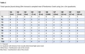
Making a table with my data was pretty straight forward. I added a totals section to my fieldwork tables and counted the number of species present in each quadrant. Transferring this information to a table was easy enough from there. After analyzing the data, made easier by line graphs of each individual transect, it was revealed to me that the pattern I was looking for was almost non existent. There were a couple of transects I sampled that seemed to support my initial observations and consequently my hypothesis that distance from the creek affects species diversity (After reading the textbook I realized I actually meant “species richness”). The majority of the transects sampled however had no discernible pattern between them. This goes to show the importance of sample size and repetition in scientific method. As far as further exploration, I would still be interested in what in what effect the creek has on species richness, but in order to find this out I would need to rethink the whole experiment and start from scratch. Perhaps requiring some comparison of near the creek vs not near the creek samples, and somehow controlling for other factors like slope, disturbance, sunlight, etc.

Blog Post 7: Theoretical Perspectives

My hypothesis touches on the effect of a stream on species richness primarily, but could actually be more related to slope or competition for resources, which may also play a factor. At this point, it appears my hypothesis is wrong however, and I believe that species richness along the stream has more to do with patch dynamics and competition for other resources other water, which I originally thought would have a stronger impact. My research will be focused on how competition for resources creates known patch dynamics along a stream, or similar waterway, in an attempt to understand the less then uniform patterns I’m observing.

Keywords might be Patch Dynamics, Species Richness, Stream-side vegetation

Blog Post 6: Data Collection

Today I began my data collection activities for my project at along D’Herbomez Creek in Heritage Park. I’ve sampled 6 out of 10 transects, each with 10-15 quadrants. In this I’ve come across  a few challenges. For one, I say 10-15 quadrants because while I intended to sample 15 quadrants per transect, some steep slopes have prevented this from occurring based on my sampling model. I’m continuing with 15 where possible but the final analysis may be of 10 to eliminate the incomplete samples from the data set. I’m finding so far that 10 should be enough to disprove my hypothesis regardless. Another challenge I didn’t foresee and perhaps should have, is the thickness of the brush in places. My initial observations saw lots of good sampling areas, but my method of randomization has sent me straight through some thickets of blackberry and other shrubs. I’ve managed but it’s definitely not the same as sampling an open field.  As far as my hypothesis, it seems to have already been disproven based on the patterns (or lack of) that I am seeing thus far. The patterns I initially observed visually, and to a lesser degree experimentally in a previous activity, don’t seem to be holding up when other, randomly chosen sites are selected. This is somewhat disappointing, but even a false hypothesis adds to our understanding.

Post 4: Sampling Strategies

In the virtual forest tutorial, a systematic sampling method, a simple randomized sampling method, and a haphazard sampling method were used to determine the frequency of seven tree species. The systematic sampling method involved randomly selecting a point along the southern margin of the study area and running a transect, straight north, through the five topographical regions (Southern Ridge Top, North Facing Slope, Bottomland, South-Facing Slope, and Northern Ridge Top). Samples were then taken from 24 quadrats (alternating between the eastern side and western side of the transect) until the northern margin was reached. The simple randomized sampling method involved generating 24 random locations to collect data. Finally, my haphazard method of sample collection involved attempting to space the quadrats in such a way that they maximized the distance between each other and the edge of the study area.

Based on the estimated sampling times, the haphazard method proved to be the fastest method (12:17 hrs) of sampling, and the simple random sampling method ended up being the slowest (12:45 hrs). However, I think it is worth noting that the systematic sampling method was, anecdotally, the fastest to conduct in the simulation and it seems logical that it should be considerably faster that either of the other two methods. This is because it covered much less walking distance than the random and haphazard method.

The two most common species in the study area were eastern hemlock and red maple. For eastern hemlock, the haphazard sampling method yielded a 6.9% error, the systematic sampling method yielded a 13.2% error, and the random sampling method yielded a 26.4% error. For red maple, the haphazard sampling method yielded a 17.0% error, the systematic sampling method yielded a 5.1% error, and the random sampling method yielded a 5.9% error.   In both cases, the systematic method was more accurate than the random method, and the haphazard varied from being the best and the worst method.

The two most rare species in the study area were striped maple and white pine. For striped maple, the haphazard sampling method yielded a 100% error, the systematic sampling method yielded a 31.4% error, and the random sampling method yielded a 42% error. For white pine, the haphazard sampling method yielded a 98% error, the systematic sampling method yielded a 185% error, and the random sampling method yielded a 49% error.   The systematic sampling method was most accurate for the striped maple; however, the random method wasn’t far off. In the case of the white pine, the systematic sampling method was extremely inaccurate and the random method was the most accurate. The haphazard method was extremely inaccurate in both cases.

Overall, the haphazard method out-performed the other methods for four out of the seven species. However, it was extremely inaccurate with determining the frequency of rare species and red maple. The inconsistent percent error values of the haphazard method lead me to believe that this method has value; however, it is a risky sampling strategy. I believe that the success from my haphazard approach is likely derived from traits that it took from a stratified method. By choosing points that were relatively far away from each other, I, incidentally, chose a similar amount of points in each region (Southern Ridge Top, North Facing Slope, Bottomland, South-Facing Slope, and Northern Ridge Top). Similarly, the systematic method performed well in most cases but had a lot of challenge with the rare species. Therefore, even though the random sampling method only outperformed both other methods in one case, it was the most consistent for determining the frequency of common and rare species.