Category: Uncategorized

Did you have any difficulties in implementing your sampling strategy?
If yes, what were these difficulties?
-Yes, the peatlands where I planned on gathering data were either flooded, or snowed over, making finding either Scotch heather or cranberry plants a challenge. The conditions have improved, however, and I returned last weekend to begin collecting data, again.

Was the data that you collected surprising in any way?
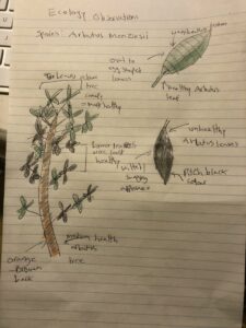
-Not really, however, I only collected one quadrats worth of data. I collected data from within the burn zone. The quadrat only contained Scotch heather (Calluna vulgaris), and it was present with 75% of the cells within a 1m^2 quadrat with 10cm^2 cells.

Do you plan to continue to collect data using the same technique, or do you need to modify your approach? If you will modify your approach, explain briefly how you think your modification will improve your research.
-My basic method of gathering data using the above mentioned quadrat will not change. However, I may change the strings in the quadrat for wires.

Also, after studying experimental design for a few weeks this semester at my own university, I have decided to make some changes to how I will design this study. I have laid my observational study as follows:

The general design format will stratified random sampling, and the the statistical analysis I will use will be based on this design. I will use Jamovi for the analysis.

The burnt area of the bog in the DND lands will constitute one sampling strata, and the unburned area around it, delineated by a square boundary, will constitute the other sampling strata. Each strata contains 10 samples, selected randomly by drawing lots (separately and independently for each strata).

After I drew these lots for each strata, I used a web application (Earthstar GeoInformatics) to figure out where these samples would be found using longitude and latitude. I generated the map shown below:

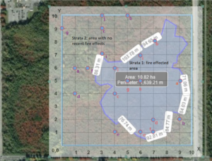
Here are the coordinates for the sample locations, and notes on how I calculated their positions:

Strata 1:

a latitude 49.17356 N longitude 123.10890 W
b 49.17538 123.10638
c 49.17493 123.10764
d 49.17265 123.10890
e 49.17129 123.10700
f 49.17356 123.10827
g 49.17493 123.10954
h 49.17175 123.10385
i 49.17402 123.10764
j 49.17538 123.10764

Strata 2:

a 49.17311 123.10385
b 49.17447 123.10512
c 49.17265 123.10701
d 49.17175 123.10511
e 49.17129 123.10574
f 49.17129 123.10511
g 49.17311 123.10638
h 49.17311 123.10575
i 49.17357 123.10512
j 49.17356 123.10701

I will use my smart phone to find each sample location.

Null hypothesis: there is no correlation between the effects of bog fire, and the presence of Calluna vulgaris and Vaccinium oxycoccos within the DND lands bog.

Alternate hypothesis: there is a correlation between the effects of bog fire and the differences in presence of C. vulgaris and V. oxycoccos, if any such difference can be observed, within the DND lands bog.

The statistical analysis I will use is summarized on this Oregon State University website. I will also be do an analysis to test for correlation between percent presence of both Calluna vulgaris, and Vaccinium oxycoccos within the burnt and unburnt strata. The presence of either species is measured by species present or not present in each cell within the quadrat, each quadrat having 100 x 10cm^2 cells.  If a species is present within the cell, this is simply considered a tally of one, for presence within cell. Both heather and cranberry could potentially be counted as present in the same cell, or they could not.

However, I’m not sure yet if Jamovi can already do this, so after doing more data collection tomorrow, I will be exploring what options that software has, and if it doesn’t, I’ll have to decided to either create a module myself, and to simply work through the mathematics myself. I should have a large chunk of my data for strata 1 collected before the weekend, and hopefully have Jamovi figured out by the end of this coming weekend.

Regardless of what modules Jamovi currently has, the sampling design I will use is what I just described, and the analysis will follow the Oregon State web page as my outline for analysis. I’ll go over this in greater detail in a future post.

Blog Post 7: Theoretical Perspectives 

In considering the patterns and productivity of fauna that predominate on two separate gradients of differing exposure to ocean climate, the diversity of the vegetative species may reflect a relationship with their environment through analysis of the piece, the soil matrix. Each gradient undergoes the consistent disturbance of winter storms that bring strong winds, large waves and heavy rainfall. An inventory of the flora might give insight towards competitive success and preferred microclimates. 

My hypothesis addresses processes of ecological disturbance through sodium ion flux influenced by environmental dynamics. These abiotic factors have extenuating contributions from rainfall and average temperatures that are not of the main focus of this study, however, are under consideration in discussion. Competition and disease may also be contributing biotic factors that are not addressed in the hypothesis, yet may be of considerable association. Statistical data is being compiled to consider resulting deductions on community structure and complexity. The frequency of storm disturbance is thought to be of primary impact on the electroconductivity of the microclimates and soil matrix from which the diversity of vegetation is based. 

 E. Carmen Bell

Blog 6: Data Collection 

On January 21, 2020, the West coast of Vancouver Island was at the tail end of a typical winter storm. The morning had seen winds of up to 33km/hr and Environment Canada expectations were 20mm of rainfall. This is not unusual, however, it was not an ideal day for data collection. The sample unit was of soil matrixes of ten replicates. Each sample underwent three tests for total dissolved solids (TDS) taken to study the conductivity of the gradients in relation to the diversity of flora species. The ten soil samples were taken from surface to a depth of fifteen centimeters. Five samples were taken from the westernmost open ocean plot (41.1331°N, 125.8905°W) and five from the easternmost inlet plot (49.1207°N, 125.8969°W). The matrix of the soil samples may be more telling as to the biodiversity as is the electroconductivity, however, I think the data I collected will provide a reasonable clear expression of the patterns of vegetation. I will add the predominant storm patterns for this time of year to the introduction of my study and wonder if it should have been incorporated into the hypothesis. 

The following is similar to Blog #5 because I have accidentally combined the two posts.  

My hypothesis is testing soil conductivity and comparing vegetative species in quadrats placed using a systematic sampling method. I maintained random selection of sample replicates by tossing my spade towards a first sample site and then used a tape measure (predetermined distance) and a compass to sample the next four sites. For each sample site in the two gradients being compared, I placed the quadrat (0.5m x 0.5m) so that the spade was in the center and in a manner that allowed for the stems of the species of vegetation present, gently discouraging vegetation that was “leaning in”.  

The soil samples were taken from surface to a depth of fifteen centimeters. Five samples were taken from the western (open ocean) plot and five from the eastern (inlet exposure) plot. The matrix of the soil samples was as I expected, the open ocean samples being mostly sand and the inlet samples being mostly humus. At home I baked each sample in the oven at 200 degrees Celsius for four hours. I used a 1:2, soil to distilled water, to create a slurry, then followed the same procedure for testing the concentration of total dissolved solids for each of the ten samples.  

Because both regions being sampled had very little differentiation, there was no need to create subareas, therefore I did not use the stratified random sample method. Instead, I used a systematic sampling method to transect the sample region, the sample sites spaced in proportion to representation of the gradient, a method that if replicated would yield samples that were also indicative of the region. The data I have collected has demonstrated completely opposite results from the position of my hypothesis. In the name of science, I will not change anything but I will explore why this is so in the discussion portion of my study. 

E. Carmen Bell

Blog Five: Design Reflections by E. C. Bell 

My hypothesis-in-the-works has shifted towards considering the soil with the highest degree of salt to have the least amount of vegetative diversity. As a result, my sample unit has become the soil in relation to flora species and visible attributes. I maintained random selection of sample replicates by tossing my spade towards a first sample site and then used a tape measure (predetermined distance) and a compass to sample the next four sites. For each sample site in the two gradients being compared, I placed the quadrat (0.5m x 0.5m) so that the spade was in the center and in a manner that allowed for the stems of the species of vegetation present, gently discouraging vegetation that was “leaning in”.  

The soil samples were taken from surface to a depth of fifteen centimeters. Five samples were taken from the western (open ocean) plot and five from the eastern (inlet exposure) plot. The matrix of the soil samples was as I expected, the open ocean samples being mostly sand and the inlet samples being mostly humus. At home I baked each sample in the oven at 200 degrees Celsius for four hours. I used a 1:2, soil to distilled water, to create a slurry, then followed the same procedure for testing the concentration of total dissolved solids for each of the ten samples.  

Because both regions being sampled had very little differentiation, there was no need to create subareas, therefore I did not use the stratified random sample method. Instead, I used a systematic sampling method to transect the sample region, the sample sites spaced in proportion to representation of the gradient, a method that if replicated would yield samples that were also indicative of the region. The data I have collected has demonstrated completely opposite results from the position of my hypothesis. In the name of science, I will not change anything but I will explore why this is so in the discussion portion of my study.

Carmen Bell

Community Sampling Exercise by Carmen Bell 

 Community: Snyder-Middleswarth Natural Area 

The three virtual sampling strategies used to assess species density for the Snyder-Middleswarth Natural Area included random, systematic and haphazard. Of the three, the area-based haphazard sampling method was the fastest at 12 hours, 12 minutes, likely because these are known representations of the larger area taken in a non-random manner. The longest duration was the area-based random or systematic method of 12 hours, 45 minutes. The difference in time between the two is not vast for the 24 plots, however, the difference may increase given more sample points.  

For the total area of the Snyder-Middleswarth Natural Area, 24 sample points were not enough to represent the diversity of the 200ha old-growth hemlock-yellow birch forest. In effect, each sample point represents 8.3 hectares (20.6 acres) over the steep terrain of a ravine created by the Swift Run River. As this is a virtual exercise, the representation can only be imagined. In a real case scenario, the accuracy represented in the sample points would depend, in part, on the variation of soil composition within the degrees of steepness. 

My assessment of the histograms from a perspective of relative species abundance, determined that the Eastern Hemlock and Sweet Birch be considered common, while the remaining species be considered rare. Within the context of biodiversity, “…, n individuals usually fit a hollow curve, such that most species are rare … and relatively few species are abundant” (McGill, et al., 2007). Each of the Yellow Birch, Chestnut Oak, Red Maple, Striped Maple and White Pine had a relatively hollow curve given the limited data. The Snyder-Middleswarth Natural Area is known as an old-growth hemlock-yellow birch forest. The lower density of yellow birch could be attributed to the larger stem size of an old growth tree. 

Considering the Eastern Hemlock and Sweet Birch as the most common species, the most accurate density reading was the Eastern Hemlock with a 10.6 percentage error between the known and sampled data. Considering the Yellow Birch, Chestnut Oak, Red Maple, Striped Maple and White Pine species as rare, the most accurate density reading lay with the Striped Maple at 14.3% error. I would like to point out that only 20 trees were sampled with a known density of 17.5. The Yellow Birch had a higher percentage of error at 30.2, however, the known density is 108.9 with 76.0 represented in sample data, demonstrating a stronger representation of the species.  

Eastern Hemlock

                 Actual   Data

520.0 – 469.9 / 469.9 x 100 = 10.6% percentage error 

Sweet Birch  

Actual   Data

188.0 – 117.5 / 117.5 x 100 = 60.0% percentage error 

Yellow Birch

Actual   Data

76.0 – 108.9 / 108.9 x 100 = 30.2% percentage error 

Chestnut Oak

Actual   Data

36.0 – 87.5 / 87.5 x 100 = 58.9% percentage error 

Red Maple  

Actual   Data

152.0 – 118.9 / 118.9 x 100 = 27.8% percentage error 

Striped Maple  

Actual   Data

20.0 – 17.5 / 17.5 x 100 = 14.3% percentage error 

White Pine

                 Actual   Data

0.0 – 8.4 / 8.4 x 100 = 100% percentage error